

During a Microsoft Excel training session a few week’s ago, I had a great question about using conditional formatting to highlight dates earlier than the current one, in other words, how can we highlight dates that occur in the past? This was a great question and so I thought I would publish a post this week about how to do this.
I have included instructions for both PC and Mac.

If you haven’t used conditional formatting in Excel before, be sure to check out my post outlining how to use conditional formatting in Excel.
On a PC
- Open the workbook you wish to apply formatting to.
- Highlight the column which contains the dates you want to work with.
- From the Home tab select the Conditional Formatting button and choose New Rule.
- The New Formatting Rule dialog box will appear:
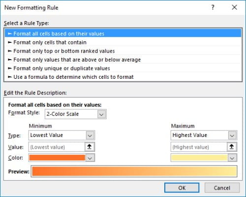
- From the Select a Rule Type, choose Format only cells that contain.
- In the Edit the Rule Description section you need to tell Excel that any cell which contains a date which is less than today’s date, highlight it.
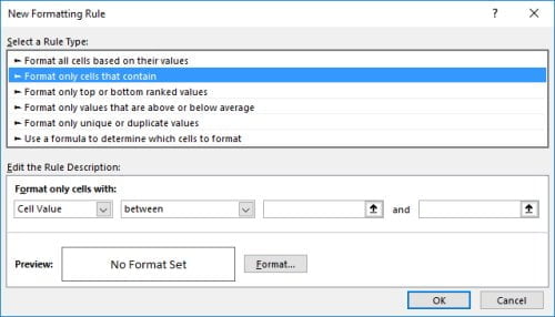
- In the Format only cells with section, leave the first drop down menu set as Cell Value.
- For the next drop down menu change it to less than as shown below:
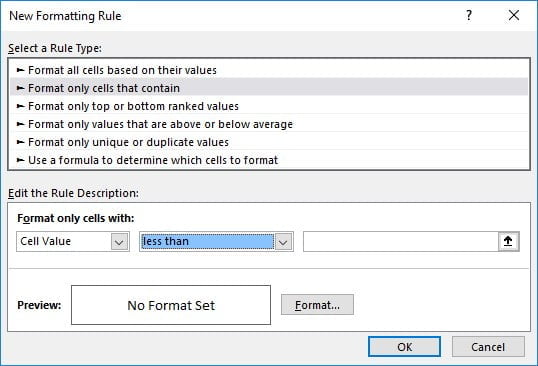
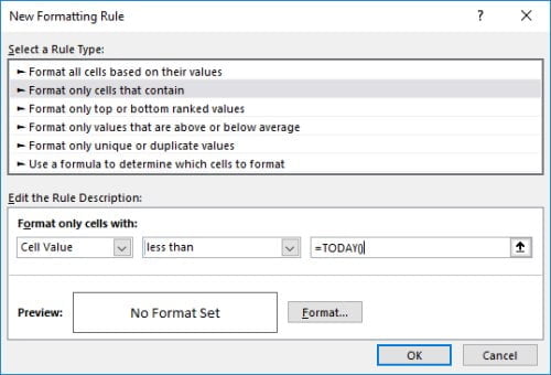
- In the formula box type =TODAY()
- This formula will look for a cell value that is less than “today”:
- Now to specify the format you want to apply, click the Format button.
- I have chosen to have the text change to Red and Bold.
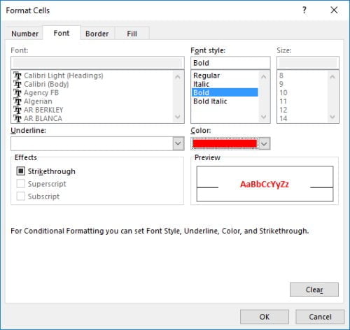
- Click OK.
- Click OK again to complete the Conditional Formatting rule.
- Any dates which occur prior to today’s date will now appear in the formatting you specified:
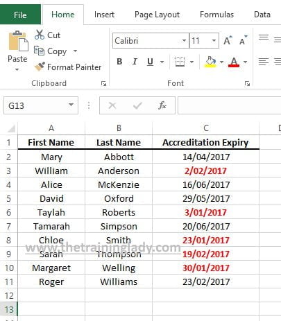
Note: For the above example, today’s date is 20 February 2017.
On Excel for Mac
- Open the workbook you wish to apply formatting to.
- Highlight the column which contains the dates you want to work with.
- From the Home tab select the Conditional Formatting button and choose New Rule.
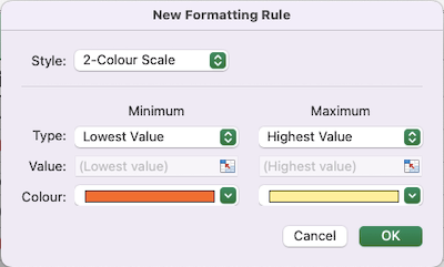
- The New Formatting Rule dialog box will appear:
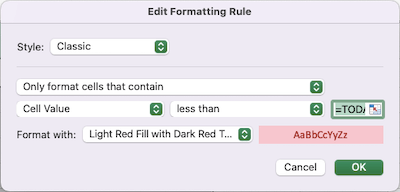
- From the Style drop-down, choose Classic.
- In the first part of the rule, choose the drop-down menu and select Only format cells that contain

- Click the drop-down containing Specific Text and change it to Cell Value
- Change the drop-down containing between to less than
- In the formula field add =TODAY()
- This formula will therefore look for a cell value that is less than “today”:
- Now to specify the format you want to apply, click the drop-down for Format with.
- I have chosen to have the text change to Red Text.
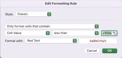
- Click OK.
- Any dates which occur prior to today’s date will now appear in the formatting you specified:
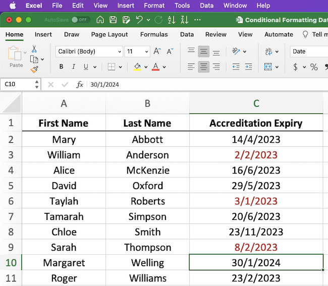
Note: For the above example, today’s date is 9 February 2023.
Want to conditional format for a range of dates?
Click here to see how you can use conditional formatting for a range of dates.
Love this article? Comment below and let me know how you’ve utilised this feature. Be sure to check out my other Microsoft Excel content here.


20 Responses
I’ve used this formula for many years, with no issues. But in the O365 version, it formats the text of cells with no dates in them. When I googled the formula and found your article, I was hoping I was going to find what changed, and maybe have a new solution. Sadly, your article uses the same formula I have always used, and the issue persists.
Hi Curt,
If there is no text in the cells then how is the formatting showing up?
If it is formatting empty cells, it will be because you have applied a Fill Color to the cell, I tend to stick with Font formatting options so that if there is no text in a cell, the conditional format is not applied.
Hi Curt, you can add an additional conditional format to the same range. “Format only cells that contain” and select “Blanks” from the leftmost drop down. Then you can just set the fill to “no colour” and that should hopefully be you. 🙂
Perfect what i was looking for.. Thanks a ton
Worked perfectly for what I needed. So grateful. Thank you.
Hi,
I have a spreadsheet that has a completed date for a task. I would like to highlight the Ref cell (Column A) green once a completed date is added to the completed column (Column O)
what is the best way of achieving this.
Many Thanks
Wakar
Hi Wakar,
Let’s assume you have text or content of some kind in column A.
Then in column O you are entering a completion date where appropriate.
Firstly you would need to apply Conditioning Formatting to just the first record, or row of data. Once the conditional formatting is created you can use Format Painter to apply it to all cells in Column A where you have data.
Select cell A2. Go to Conditional Formatting and choose New Rule.
Now select “Use a formula to determine which cells to format”.
Into the field type =O2>0.
This will mean Excel will check cell O2 and as long as SOMETHING is in that cell, it will change the formatting of the current cell, cell A2.
Click the Format button and apply a Font Colour and maybe BOLD if you like.
Click Ok to finish choosing the format and OK again to complete the conditional format.
Add a date into cell O2. The format of whatever you have in cell A2 should now change.
If you delete the date from cell O2 then the formatting is removed.
For help on applying the conditional formatting using Format Painter, see my post on applying conditional formatting to an entire row, it is the same concept however you only want the formatting to appear on 1 x cell instead of all cells in a row.
https://www.thetraininglady.com/conditional-formatting-entire-row/
Hope this helps.
Hi
I have a column of dates that courses were complete. I would like to highlight dates in another column that are due for renewal 6 weeks prior to the expiry date in a year’s time in orange and also in the same column, the expiry date will show up in red. Is this possible with conditional formatting?
Many thanks
Loraine
Hi i would like to ask for your help.
I want to use conditional format for the following case:
1. =($G14=10 …. if the days in $G14 are less than 10 days (expiring items) to be orange color the cell
Where is my mistake ?
Because all cells with dates older than TODAY are green. No orange color
Hi Harris,
Sorry for the delayed, only just saw your question.
If column G has numbered which are the number of days till something expires then we can conditional format column G so that any value that is “less than or equal to” 10, make the cell go orange.
Follow these steps:
1) Highlight column G and select Conditional Formatting > New Rule
2) Choose “Format only cells that contain”
3) From the options within the rule ensure you have “Cell Value” selected and then change the “between” to be “Less than” from the second drop down
4) In the last field enter 10 as this is the criteria you wish to use
5) Now click the Format button to tell Excel which formatting to use when highlighting values which meet your criteria
6) Choose the Fill tab and select an orange colour then click OK
7) Click Ok twice more times
8) Any value which is less than 10 should now be highlighted in orange
Hope this helps.
Belinda
A formula produces a date in cell A1
Conditional formatting on A1 to determine if A1 is < today() or not….. FAILS.
Assume A1 = 3/30/20
Assume today() = 3/24/20
Conditional formatting on A1 should produce no change because the criteria was not met (i.e. < today() ). But it DOES produce the format change reserved for date is less than today() being true (a strike through)
Assume A1 = 3/20/20
Assume today() =3/24/20
The format change to strike through occurs……..although since it occurs regardless, I don't consider that much of a test.
I'm new to Office 2019…………….what I wish the conditional formatting to do worked fine on Office 2003, but fails on 2019. Clearly there is a flag somewhere that I am not setting properly.
Any help would be appreciated
This is probably of no help to you, but in case someone else has the same issue.
Whenever conditional formatting doesn’t work as expected, check the rule to make sure it’s actually what you typed. Excel likes to be “helpful” and will do silly things like change =today() to =’today()’ or change A1 to A1048576. I’ve no idea why it does it, just that it does sometimes.
I’ve searched & searched & hope you can help…
I have a column with various due dates. I want the due date cells to highlight 15 days before the date entered (sort of a warning that the due date is coming up). So if I have a due date of 5/15/2020, i would like the cell to change colors on 5/1/2020, etc. Is there a way to do that?
Thanks so much!
Hi Jenette,
This is a great question and one I have had a few times. So I’ve written you a full post with the instructions on how to do this. You can view it at https://www.thetraininglady.com/conditional-formatting-dates-range/. Let me know how you go.
Thanks, Belinda
How can you ignore blank cells with this formula?
thanks
Hi Maria,
Because this is achieved using Conditional Formatting, and not an actual formula we are unable to have it ignore blank cells. If you only apply font based formatting such as bold text, or change the font colour, the blank cells will not change in appearance. If however, you apply formatting such as a Fill colour then blank cells will also be formatted. Simple switch the formatting type over to just the options on the Font tab within the Format Cells dialog box and you should have no formatting being applied to blank cells. Hope this helps.
Belinda
I tried several other search results, none of which worked. This is the only one that actually worked and was simple to do – thank you!
Thank you Michelle for the feedback. So glad to hear it worked and was simple. 🙂
Hi this is a great help but I want to add a second condition to clear when the task is completed by another cell having a Y entered in it – how do I do that please? (I don’t even know the terminology to look it up I’m afraid)
Hi Sally,
From what you have written I think you could use a combination of an IF statement and then conditional formatting to achieve what you are after. If you’d like to send a screenshot of your workbook to info@thetraininglady.com I’m happy to take a look at it and give you some details, or even upload a post to the site with instructions on how to achieve what you are after.
Thanks,
Belinda
aka The Training Lady