Do you know how to create a Vlookup in Excel? The Vlookup function in Excel is a very popular function but sometimes can be a little tricky to work out. The Excel Vlookup function is a fantastic time-saver as it is a perfect example of how Excel can “do the work for you”. The Vlookup function allows you to have Excel look at a value, then go and find corresponding information based on that value from a table within the workbook.

This Vlookup tutorial will solve any confusion you have about using the Vlookup function and provide you with some tips to master it like a pro.

Examples of a Vlookup

Below are some great usage examples of the Vlookup function:

• Look up a staff or student ID and respond back with related information such as DOB/Age, phone number, email address, class details etc.
• Look up a product code and respond back with product name, weight, size, supplier, cost price or RRP, stock information and so forth.
• Look up a number based score and respond back with the correct grade for that score.
• Anything where you want to find a value from a larger set of information (called a table) and return a corresponding value from within that table…

When to use a Vlookup?

Anytime you have a table of data where you need to lookup one value to find a corresponding value, you can use the Vlookup. The Vlookup function is used when the table of data you are looking up from is presented in a “vertical” layout. Column 1 must have the lookup values, column 2 and so on will have the addditional information you can return back.

There is also a Hlookup function. The Hlookup is when your data is presented in a “horizontal” layout. Both functions provide the same end result but provide the flexibility of having your data table in whichever layout you prefer.

Vlookup Syntax

An important part of understanding any function in Excel is understanding the parameters required. The way that a function looks and what information needs to be entered in which location is defined by the syntax.

Here is a look at the Vlookup Syntax:

=VLOOKUP(lookup_value, table_array, col_index_number, [range_lookup])

Lookup_Value	The lookup value is the cell reference containing the value you wish to lookup.
Table_Array	The table_array is the location of the data containing the answer you wish to lookup.
Col_Index_Number	The col_index_number is the column number within the table_array where the answer will be found.
Range_Lookup	The range_lookup tells Excel which type of matching to use: find the closest match, or an exact match.

Create a Vlookup

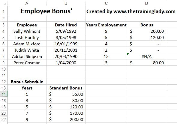
In our first example, we are using an employee bonus schedule where we want Excel to look at the number of years each staff member has been employed, then go to our bonus schedule table, which is laid out in a vertical format, and identify how much each employee will receive as a bonus based on their years of employment.

In this example I’m only looking at 6 staff members so technically I could manually look these up myself. Imagine though if I had 500 employees – it would be very time consuming if I did this manually. This is where the Vlookup is going to save ALOT of time.

To create an Excel vlookup function, follow these steps:

1. Open Microsoft Excel.
2. If you wish to use an existing file which contains a table of data suitable for this exercise, press Ctrl + F12, the Open dialog box will appear allowing you to locate the file and click Open.
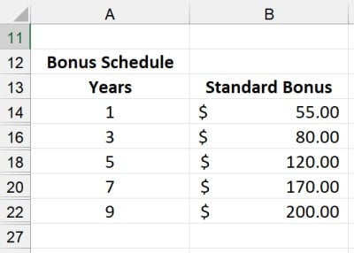
3. If you do not have an existing file, create a sample file such as the one shown below:

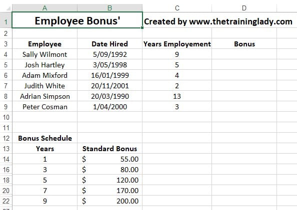
4. From the sample above you can see our Bonus Schedule table is displayed in cells A14:B22.

TIP: In a real-world scenario I would recommend having your table of data on a separate worksheet, separate from the data you wish to lookup.

5. Place your cursor in cell D4.
6. We will use the Function Wizard to provide some guidance for new users.
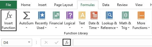
7. Select the Formulas tab and click the Insert Function button OR click the Insert Function button located on the Formula Bar:

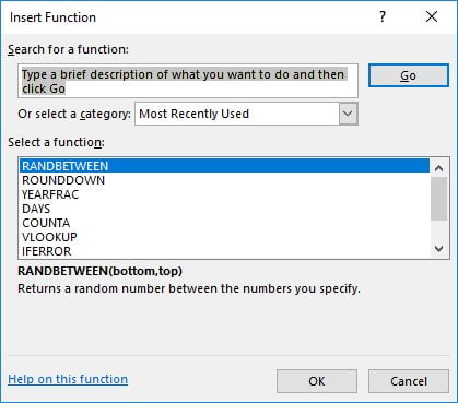
8. The Insert Function dialog box will appear:

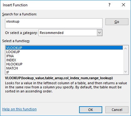
9. In the Search for a function box type the function name (in this example, type vlookup) you are searching for, or if you are unsure which function to use, type in a description of what you wish to achieve, then click Go.
10. A list of functions which are applicable will be displayed:

11. By clicking on each function displayed you can read a description for each below the list.
12. If you are attempting to use a new function, click the Help on this function link in the bottom left of the dialog box, this will give you a full overview of the function and how it can be used.
13. Select Vlookup from the list and click OK.
14. The Function Arguments dialog box will now appear:

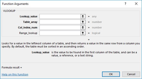
15. Place your cursor in the Lookup_value field; within this field, we must select the cell which contains the value we want to “lookup”.
16. This field has the Collapse dialog box button on the right side which means that Excel will allow you to use the mouse and select any cell on the worksheet, if the dialog box is blocking access to the cell you need to click on, click the Collapse button otherwise, just leave the entire Function Arguments dialog open and select the correct cell:

17. Click and select cell C4.
18. Now move your cursor to the table_array field.
19. You must now select the location of your table data, be sure to only select the cells which contain data, do not include the headings.
20. Select cells A14:B22.
21. Because we will be using AutoFill to copy this function to other cells, place your cursor within the A14 reference and press F4 on the keyboard once to make the reference “Absolute”. Repeat for the B22 reference.
22. The Table_array should look as follows:

23. Move your cursor to the Col_index_number field.
24. You must now enter the numerical value of the column you wish to retrieve the match result from.
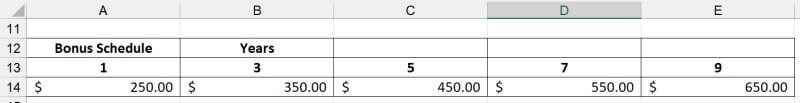
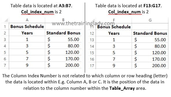
25. In this example, we want to return the value of the bonus amount. It is important to use the value of the column within the table data and not the column number within Excel. See the examples below:

26. Enter the value 2 into the Col_index_num field.
27. Now move your cursor to the range_lookup field. This field determines if you want Excel to find you the closest match or an exact match.

Info: You will notice in our table_array that only the years where an employee will receive a bonus are listed. Year 2, 4, 6 and 8 are not listed in the table as employees do not receive a bonus in these years. If you leave the range_lookup field empty, Excel will find the nearest match, meaning that employees who have been employed for 2, 4, 6 and 8 years will still receive a bonus when they should not. To avoid this issue you can use the range_lookup field to tell Excel to find only an Exact match.

28. In the range_lookup field type False:

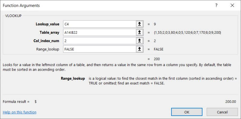
29. Click OK.
30. The answer $200 will be returned as the bonus amount for the first person in my example.
31. You can double-check the answer by looking up the bonus amount for 9 years of employment, which is $200.

AutoFill the function

There is no need to repeat the process to create the vlookup function again. Use the AutoFill feature to copy the formula to other cells. Because we used absolute cell referencing (the dollar $ symbol in the cell references for the bonus schedule table), we can AutoFill this and our answers will be accurate for all employees. It is worthwhile having a go at a few of the examples yourself so that you get more than one practice using the Vlookup function – remember practice makes perfect!

1. Select cell D4.
2. Place your cursor on the bottom right corner of the cell till the mouse cursor changes to a +
3. Hold down the left mouse button and drag down to the bottom of cell D9 and release the mouse button.
4. The function will now be copied down the column:

What about the errors?

You spot them too? The #N/A error for cell D8 is in fact Excel telling you that there was not an exact match for those particular values. The value being looked up is 13 years of employment, our Bonus Schedule table only goes up to 9 years of employment, therefore, Excel has responded with an error message. A common question I hear is: “I don’t want errors on my spreadsheet, how can I make this look better?”.

Here is my tip to fix this and make your spreadsheet look better.

1. Adjust the table_array area to include ALL possible answers. In this example, add entries for years 2, 4, 6, 8, 10, 11, 12 etc. In the bonus amount simply enter $0:

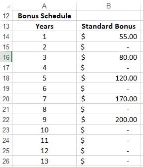
2. If you do not wish to have these additional years displayed, hide the rows and leave only the rows with value amounts displayed. You can see below that rows 15, 17, 19, 21, 23-26 are hidden on the worksheet:

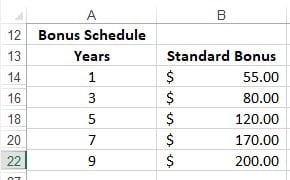
3. You may need to adjust the table_array cell references within the Vlookup in case it does not automatically acknowledge these new entries.

You have now completed a basic vlookup function in Excel. Be sure to check out other great posts for Microsoft Excel. Comment below with any questions or share how you use a Vlookup in your spreadsheets.