

It seems my conditional formatting posts have become quite popular and with that, I’ve had some amazing questions asked about variations of how to use conditional formatting. One such question was how to apply conditional formatting to an entire row in Excel. The approach for this one is a little bit different but works amazingly.
If you haven’t already taken a look at my other conditional formatting posts, be sure to explore how to use:
- conditional formatting with dates based on a range,
- conditional formatting based on dates earlier than today.
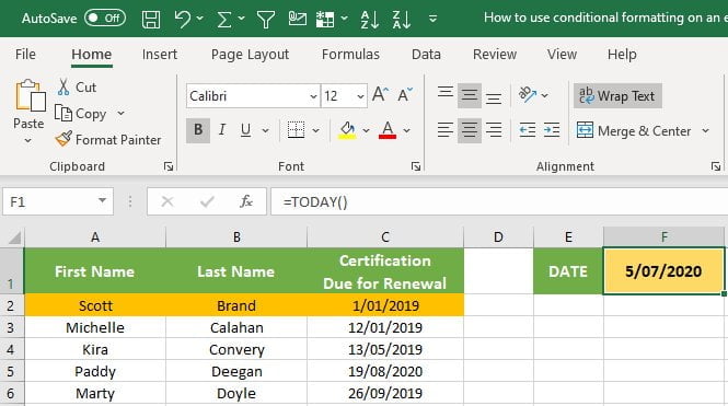
First off I have my list of names along with dates that staff are due to renew their certifications. I am going to set up Excel so that it highlights the entire row of data when a date has passed todays date.
- Open the sample file you wish to use, or recreate a sample similar to the one shown below:
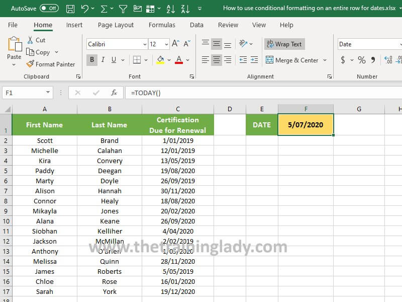
- I have added the =TODAY() formula into cell F1 which I will reference in the conditional formatting. This gives me the flexibility to easily change this date depending on my needs and the conditional formatting will automatically respond and change formatting where applicable.
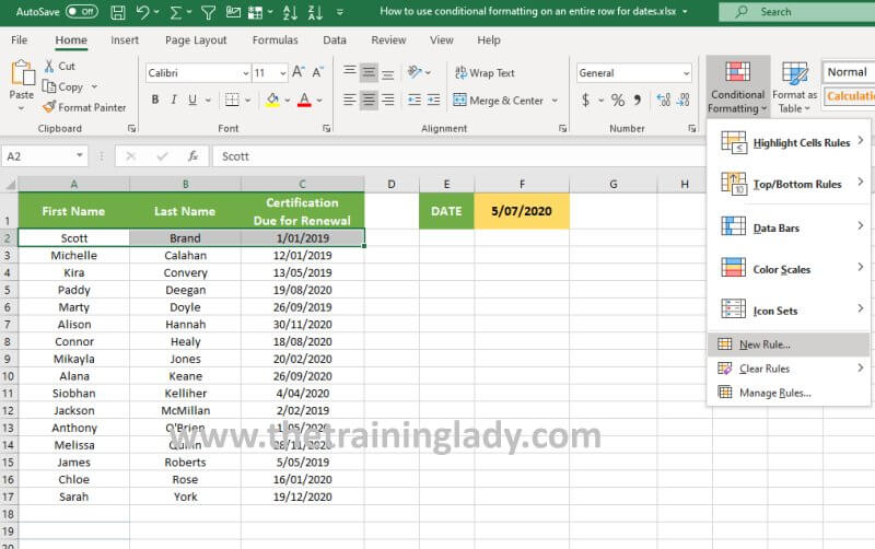
- Now we are going to create the new conditional formatting rule on the first record only.
- Highlight cells A2 to C2.
- From the Home tab select Conditional Formatting > New Rule:
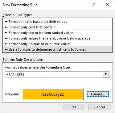
- From the options, select Use a formula to determine which cells to format:
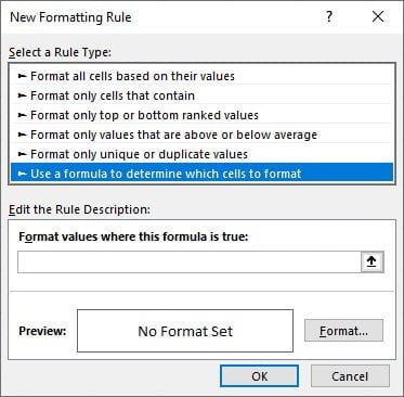
- Now in the Format values where this formula is true, we need to create a formula which will check the dates for us.
- Into the field type =$C2<$F$1
- Here I have used absolute cell references to lock only the column letter for C2. We will be copying this formatting to the other rows in our worksheet so I want the row number to be relative so that it changes with each row we copy this to. I do not want the column letter to change. I have then locked the entire cell reference looking at our date cell in F1.
- Now click the Format button and apply either Font formatting, or Fill formatting options:
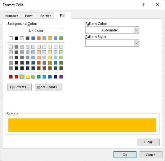
- Click OK once you have selected the formatting you wish to use.
- Click OK to complete the rule:
- Click OK again to close the New Formatting Rule window.
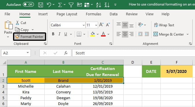
- My first example record meets the criteria of being a date earlier than today so it has formatted accordingly (in gold):
- Now I need to use Format Painter to apply this same conditional formatting to the other records in my worksheet.
- Highlight cells A2 to C2 and click the Format Painter button from the Home tab:
- Now select the remaining records in your worksheet where you would like to use the conditional format.
- All records which meet the criteria should now be formatted accordingly:
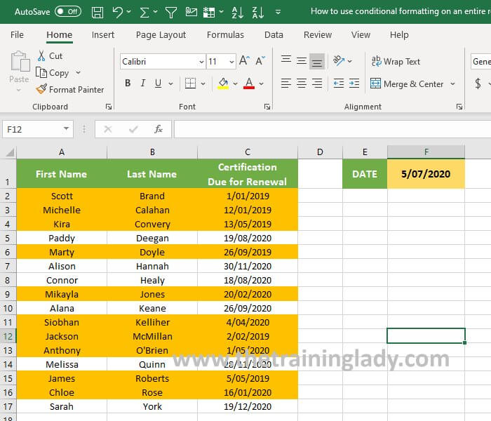
- If you want to test out the formatting, change the date used in cell F1 and your record formatting should respond accordingly.
- Have fun!
Every time I run an Excel course (which is often), I always say how much fun Conditional Formatting is. This just shows yet another genius way to use the program in a way that those visually minded users can appreciate.
If you are Sydney based and interested in having me come to your workplace for some training feel free to make contact otherwise check out my other great Excel based articles here.