How to create an Excel drop down list

Ever seen an Excel drop down list and wondered how on earth to create it yourself? Look no further as you’ll be on your way in 5 minutes to creating as many drop down lists as you want.

An Excel drop down list provides several advantages within a workbook. Not only can you control how data is entered into your worksheet, but you also limit the use of abbreviations or values which should not be included. A simple drop down list provides users with a set list of items to choose from and Excel will ensure that no other values can be entered.

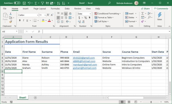
In the example below there is no consistency in the way data is entered into the Source column (column F) or the Course Name (column G) column which will make sorting and filtering difficult in the future.

Let’s look now at how we can create an Excel drop down list to allow users to select from a pre-defined list of options. In my example, I want to have a column in my worksheet where users must select from a list of specific locations.

Create the list items

To create the drop down list we are going to use the Data Validation tool. This allows you to specify the type of information you wish to have entered into a cell, row or column.

1. Open Microsoft Excel.
2. If you wish to work on an existing file then press Ctrl + F12 to display the Open dialog. Locate the file and open it.
3. If you want to start from scratch you can work directly from the new blank workbook displayed.
4. We will use the first blank worksheet (Sheet1) as our main data entry sheet. We will need a second worksheet to store the options we want to be displayed in the drop down list.
5. Click the New sheet button at the bottom of the window:

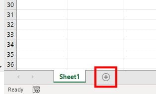
6. A new blank worksheet will be added.
7. Click on the new worksheet to open it, this will hold the options to be used in our drop down list.
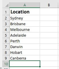
8. In cell A1 type the heading Location.
9. In cell A2 type the first location e.g. Sydney.
10. Press Enter and continue to add approx 6-8 different locations into the list.
11. You can format the heading as needed and resize the column if you prefer. You can even use the Sort function to put the list into alphabetical order:

Display the drop down list

Now that you have created the list of items you want included in the drop down menu, you can now specify where the Excel drop down list will appear.

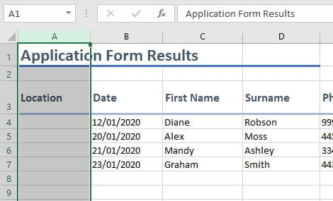
1. Return back to Sheet1.
2. Type the heading Location into an appropriate location.
3. Highlight all of column A by clicking once on the column heading:

4. Select the Data tab from the Ribbon.
5. Click the Data Validation button and choose Data Validation from the drop-down menu:

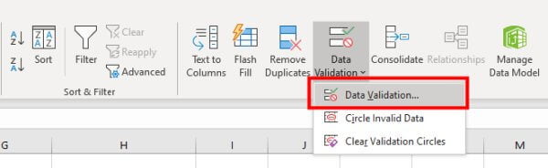
6. The Data Validation dialog box will appear:

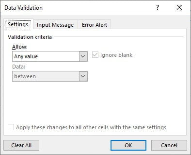
7. From the Allow drop-down, select that you want to allow a List.
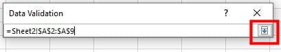
8. You now need to select the location which holds the list within the workbook.
9. Click the Collapse button on the right side of the Source field:

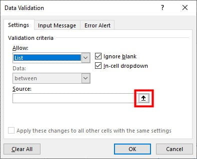
10. Highlight the cells which hold the list items you want displayed in your drop down list.
11. Select Sheet2 and highlight the cells containing each location, do not include the heading (I’ve highlighted A2:A9):

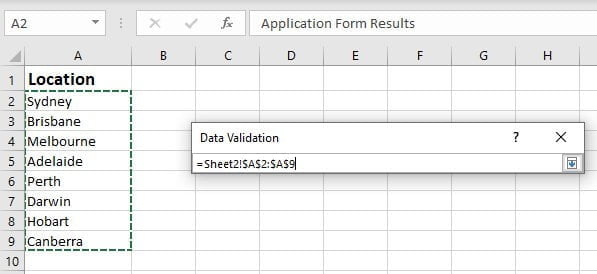
12. Click the Expand button to bring the Data Validation dialog box back:

13. Click OK.
14. Place your cursor in column A and you will see a drop-down arrow appear on the right side of the cell:

15. Click the drop-down list and select a location.
16. Your list will now be available for the entire column.
17. Repeat this process to create drop-down lists in any other columns within the workbook.

Edit an Excel drop down list

If you need to add additional options to a drop down list, or you’ve made a spelling error, you can easily edit the list within the worksheet.

If you need to edit an option within the list:

1. Open the second worksheet which contains all the list items you have created.
2. Edit the entries as normal.
3. The edited entries will now be available via the drop down lists on your data entry worksheet.

To add more options to a drop down list:

1. Open the second worksheet which contains all the list items you have created.
2. Add in any additional options you wish to include.
3. Go back to your data entry worksheet.
4. Highlight the column containing the corresponding drop down list.
5. Select the Data tab from the Ribbon.
6. Click the Data Validation button and choose Data Validation from the options:

7. Edit the Source field by clicking the Collapse button:

8. Highlight the new range of cells containing your list options.
9. Expand the dialog box again and click OK.
10. Your new list items should be available through the drop down list in your data entry worksheet.

To remove a drop down list

If you no longer wish to use a drop down list in your worksheet, you can easily remove it.

1. Highlight the column containing the drop down list.
2. Select the Data tab from the Ribbon.
3. Click the Data Validation button and choose Data Validation from the options.
4. Change the Allow field to Any value:

5. Click OK.
6. The column will now allow any type of value to be entered.

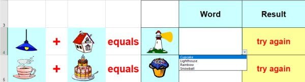
This is also a great feature for use within a classroom setting. Teachers can create interactive quizzes allowing students to choose an answer from a drop down list. This can be extended to include a self-marking function to let students know if the answer is correct or incorrect.

For more Excel tips and tricks check out more Excel posts.