I can hear you asking it now, what is a Sparkline? It’s a very good question which I’m going to answer for you now.

Sparklines were introduced in Excel 2010 and are a great feature for those who prefer a “visual” approach to data (like myself). Sparklines are miniature charts which are displayed within a cell and can show trends within your data. The advantage of using a Sparkline instead of a chart is that instead of having a chart take up half your worksheet you can incorporate a Sparkline into a single cell allowing you to visualise a row or column of data at a time.

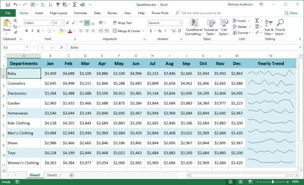
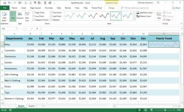
Below you can see my example of data with sparklines being used in column N.

Microsoft Excel gives you the ability to insert three (3) different types of sparklines: Line, Column and Win/Loss. Which type of Sparkline you choose will depend on the type of data you are using and how you wish to display the information.

It is important to be aware that because Sparklines are a feature of Excel 2010 and above, you cannot view them if your Excel workbook is opened in earlier versions of Excel. Likewise, you will be unable to insert a sparkline if your current workbook is running in Compatibility Mode. To find out how to convert workbooks from older versions to the latest file formats, see my post Convert workbooks to the latest file format in Excel.

Create a Sparkline

To create a sparkline, follow these steps:

1. Open Microsoft Excel
2. Open an existing file containing data you can use to add a sparkline (Use Ctrl + F12 on the keyboard to bypass Backstage view and go directly to the Open dialog box) or just create a quick sample of data
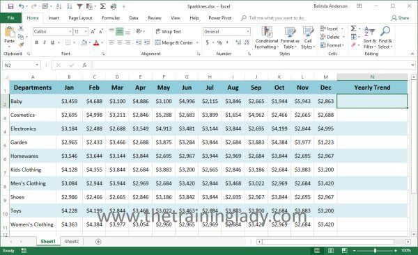
3. Place your cursor in the cell, where you wish to insert the Sparkline, I have selected cell N2

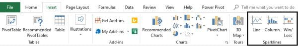
4. Click the Insert tab from the Ribbon
5. From the Sparklines group click Line

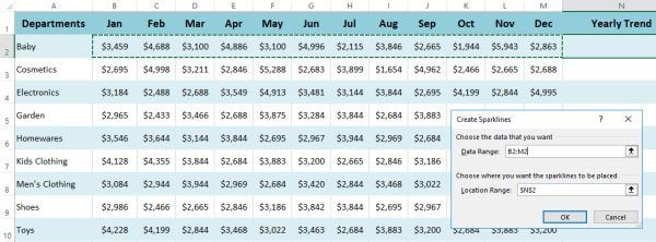
6. The Create Sparklines dialog box will appear:

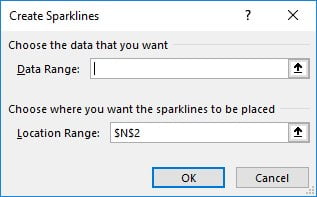
7. The Location Range has already been filled in as the cell you had selected. This will be the location the sparkline will be placed.
8. Now you need to select the Data Range you wish to include in your Sparkline
9. Use your mouse and highlight the data using the left mouse button

TIP: You can also perform this action in reverse; instead of selecting the cell where you want the Sparkline displayed, highlight the data instead and then select Insert > Line. You will then just need to select the Location Range (cell) you want the actual sparkline to appear in.

10. Once you have completed this step click OK
11. The Sparkline is displayed in the cell:

12. You can now use the AutoFill tool to fill this sparkline down the column where appropriate. If you are not familiar with the AutoFill tool, see my article here.

Sparkline Groups

When using the AutoFill tool to create the remaining Sparklines, you will automatically create a Sparkline Group. A Sparkline Group means that any changes you make to one Sparkline, will automatically be applied to all Sparklines in the group. This is very useful if you want to keep the styling of your Sparklines the same. If you want to use different Sparkline types and styling for each Sparkline, you will need to either create each Sparkline individually or ungroup the Sparkline from the group.

Now that you have created some basic Sparklines, let’s look at how you can “jazz” them up and customise the look of these nifty little critters by checking out how to Customise a Sparkline in Excel.