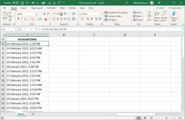
Last week I received an SOS from a good friend. She had data that was exported from an LMS and being used for analysis within Excel. A particular column contained a date and time in each cell that needed to be filtered and sorted by month. This was proving impossible as the data was being treated as text rather than Excel recognising the date formats. So how on earth can we convert the text to a date format?

To sort out this situation we needed to use two different methods: Text to Columns, and Filtering.

Separate data using Text to Columns

One of the great features you can utilise when trying to clean up data in Excel is the Text to Columns feature. This tool allows you to specify a specific delimiter such as a tab, comma or semicolon and use the delimiter to identify where your data should be split. This results in data that may have been located within one column, separating and being displayed across 2, 3 or more columns.

The first thing we are going to do is separate the date and time information which is delimited by a comma.

1. Highlight the column containing the data you wish to split
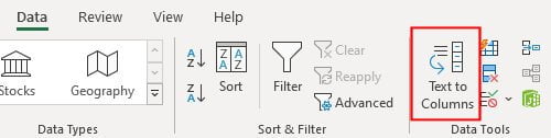
2. Select the Data tab and choose Text to Columns

3. The Convert Text to Columns Wizard – Step 1 of 3 window will appear:

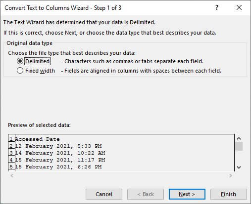
4. Make sure that the Original Data Type is set to Delimited
5. Click Next
6. In this particular example, the date and time are separated by a comma, so I will select the Comma delimiter type and untick the Tab delimiter:

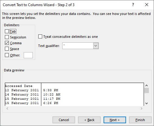
7. You will see the Data preview window at the bottom shows a dividing line appears between the date and time data
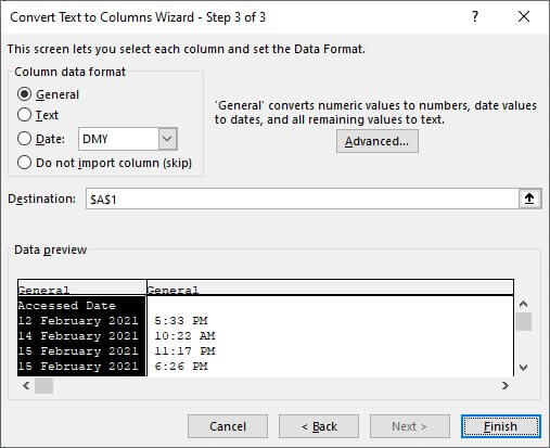
8. Click Next
9. The final step of the wizard asks what data format you’d like the new column to use, leave it as General and click Finish

10. The date and time is now split into separate columns

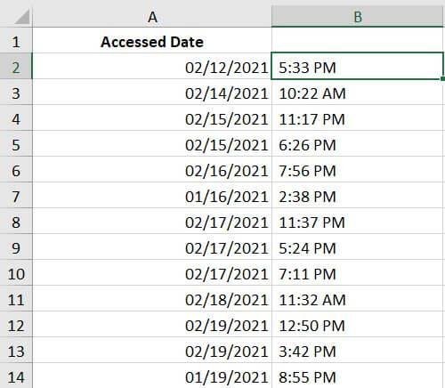
11. Automatically Excel recognised the dates and has formatted them as such
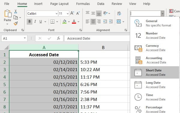
12. In my example, the dates are automatically using US date formats, I’m in Australia so I want these showing in our date format
13. Highlight the column containing the dates
14. From the Home tab click the Number Format drop-down menu and choose Short Date or Long Date format

15. The date formats are now corrected

Filter dates by month

Now that I’ve cleaned up the data set, I can now use the Filter functions within Excel to filter out dates by specific month.

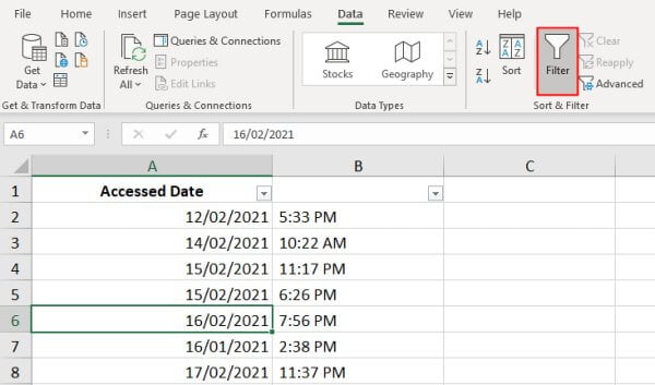
1. Click within the data area and click the Data tab and turn on the Filter button
2. The Filter drop-down arrows will appear on each column of data

3. Click the drop-down arrow for the column you wish to filter by month
4. You will see the records are shown grouped into year and month options

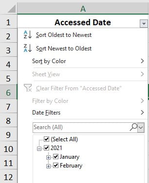
5. Remove the tick from the months you do not want to include in your filtered data set. I only want to see records for January 2021, so I untick the February checkbox and click OK
6. I can now only see records from January
7. Your data is now filtered by month
8. To bring all data back, or remove the filter, go back into the drop-down menu for the column you have filtered
9. Click Clear Filter From … from the options

I hope this has helped to understand how to use the Text to Columns function and perform a basic filter based on dates within Excel. If you have any questions or comments please post them below.